In my previous post, I highlighted the growing influence and adoption of Artificial Intelligence (AI) and machine learning (ML) systems, discussing how they attain “intelligence” through a careful “data diet.” However, a fundamental challenge arises from out-of-distribution (OOD), posing barriers to robust performance and reliable deployment. In particular, covariate shift (eq 1) and concept drift (eq 2) are two major types of OOD frequently encountered in practice, demanding mitigation for robust model deployment.
\begin{equation} \begin{aligned} \text{Covariate shift:} \quad P_\text{S} (X) \neq P_\text{T} (X) \end{aligned} \end{equation}
\begin{equation} \begin{aligned} \quad \text{Concept drift:} \quad P_\text{S} (Y | X) \neq P_\text{T} (Y | X) \end{aligned} \end{equation}
In this post, we delve into strategies to tackle OOD and enhance the robustness of AI/ML models.
1. Baseline: Quality Control and Normalization
In various discussions today, people often talk about data quality, batch/cohort effects, or “garbage in, garbage out”. These are actually quite relevant to robustness of your model. As a result, the first thing we should consider prioritizing is to establish quality control in your data generation/collection pipeline and to conduct data normalization. For scenarios prone to data biases (e.g., batch effects in biological experiments), designing control measurements becomes crucial for later data normalization. Quality control and normalization ensure that the data’s quality is suitable for model training and inference, and that the inputs are on comparable scales.

Fig 1. Quality control and normalization workflow adopt in digital pathology. Prostate (a) and lung (b) tissue images stained with hematoxylin and eosin were normalized against target images and evaluated by pathologists. Source image is from Fig2 in Michielli, et al (2022).
Fig. 1 illustrates a clinical workflow in digital pathology. Despite variance in stain levels and random artifacts, stain normalization significantly improves image quality and enhances clinical diagnostic confidence (Michielli, et al (2022)). When developing and deploying computer vision (CV)-based AI/ML systems for assisting pathologists, stain normalization and quality controls help mitigate covariate shifts in the stain images. In other words, after these data preprocessing steps, the marginal distribution of images in source and target domains becomes comparable. Consequently, OOD problems transform into IID ones.
$$ \text{Biases} \xrightarrow{\text{e.g. batch effects}} P_\text{S} (X) \neq P_\text{T} (X) \xrightarrow[\text{QC}]{\text{normalization}} P_\text{S} (X’) = P_\text{T} (X’) $$
2. Domain Adaptation when Target Domain is Accessible
2.1 Instance-Reweighting
Despite our efforts in quality control and normalization, covariate shifts may persist. Such situations often indicate selection bias, where samples from the source domain may not cover all possible feature distributions, failing to fully reflect the target domain. While acquiring less biased or more representative data seems intuitive, it can be prohibitively costly in terms of both money and time, often requiring cross-functional efforts over months to years. Consequently, computational tactics or mitigations become essential and may prompt inquiries from managers or even CxOs.
To address this, let’s begin by checking for any known information about the target domain. The observation of covariate shifts implies some knowledge about the target domain, such as the statistical distributions of features. This information becomes valuable for guiding the use of source domain data to build a model that performs well in the target domain. Such a goal is also known as domain adaptation, because the aim is to adapt the model trained on the source domain to generalize effectively in the target domain with different distributions.
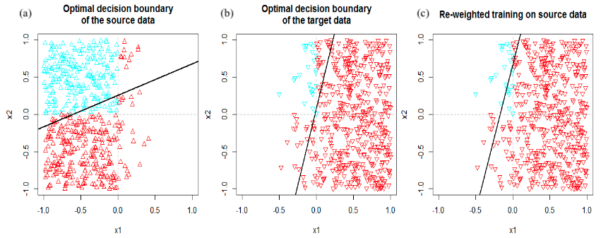
Fig 2. Instance-reweighting adapts the classifier trained in source domain to generalize to target domain. Source images are from Jong (2017).
Instance-reweighting is a domain adaptation method leveraging the target domain distribution. To illustrate, I just use the great examples from Johann de Jong’s blog. Fig. 2 displays the distributions of features x1, x2, labels of each data point, and learned and ground truth decision boundaries. Due to selection biases, the source domain exhibits different marginal distributions compared to the target domain (Fig. 2a). Training a classifier solely on source domain data yields a decision boundary diverging from the ground truth for the target domain (Fig. 2b). Instance-reweighting involves adjusting each training instance’s weight in the source domain to match the target domain distribution (Fig. 2c). This reweighted training significantly improves the learned decision boundary’s performance in the target domain. Instance-reweighting is widely adopted when instance-specific considerations are needed for model training and evaluation. For example, addressing problems with long-tailed distributions involves static reweighting (constant sample weights) or dynamic reweighting (e.g., via focal loss 1) to penalize minority groups more, resulting in more robust performance against rare events.
In summary, instance-reweighting aims to mitigate encountered covariate shifts by adjusting the sample distribution. With the reweighting scheme matching the target domain, the reweighted source domain distribution $P_\text{S}’ (X)$ aligns with the target domain distribution $P_\text{T} (X)$.
$$ \text{Biases} \xrightarrow{\text{e.g. selection biases}} P_\text{S} (X) \neq P_\text{T} (X) \xrightarrow{\text{reweighting}} P_\text{S}’ (X) = P_\text{T} (X) $$
The additional knowledge used to derive the weights introduces some inductive bias for the model; thus, the accuracy of this additional knowledge about the target domain can be critical to the model’s robustness.
2.2 Semi-Supervised Learning
In addition to target domain statistics, if we have access to unlabeled data from the target domain, we can explore other domain adaptation methods leveraging the intrinsic structure behind the data to improve OOD performance. For instance, employing a semi-supervised learning algorithm allows incorporating unlabeled data from the target domain during model training. The initial model is trained based on the source domain data. Subsequently, this model is applied to the unlabeled target domain data to generate pseudo-labels for those unlabeled samples. Samples with confident pseudo-labels are selected as additional training data, and the model is retrained alongside the source domain samples. This iterative process refines the model, enhancing its performance in the target domain.
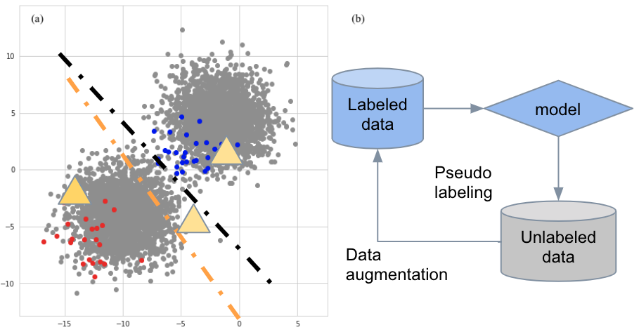
Fig 3. Semi-supervised learning aids domain aptation. (a) Massive unlabeled data representing the target domain is useful to overcome selection biases in the source domain and assist the model in generalizing to the target domain. (b) Pseudo-labeling algorithm iteratively augments the source domain data and regularizes the model training.
2.3 Test-Time Training
Additionally, Test-Time Training (TTT) (Sun, et al (2020)) can be explored even when there is no access to the target domain until running model testing. This technique introduces additional self-supervision tasks that can be applied to unlabeled data from the target domain. In an image classification task example as shown in Fig. 4, the model first projects the images into a latent space via an encoder. Then, the latent representation will be used for predicting the rotation angle of the images in addition to predicting the object label of the images. Self-supervised targets can be easily obtained since you know the angle at which the image is rotated in the data-augmentation process. During testing, we now have access to the target domain data as it is input for the model for making predictions. Each test image can be augmented via rotation and passed to the model for self-supervised learning. This self-supervised learning offers a chance to update the encoder based on the target domain, which learns how to project the target domain images into a comparable latent space relative to the source domain. This is the test-time training.

Fig 4. Test-Time Training. Source image is from the authors’ page (link) of TTT (Sun, et al (2020)).
Both semi-supervised learning and test-time training alleviate covariate shifts by seeking data augmentation to get equivalent IID.
$$ \text{Biases} \xrightarrow[\text{batch effects}]{\text{e.g. selection biases}} P_\text{S} (X) \neq P_\text{T} (X) \xrightarrow[\text{self-supervised regularization}]{\text{data augmentation}} P_\text{S} (X’) = P_\text{T} (X) $$
While these are effective methods and tactics in many real-world applications, there may be other factors limiting their adoption. For example, in scenarios with strong regulations, such as when the deployed model needs to be fully locked and requires FDA approval, using the target domain data (e.g., clinical trial data and samples collected post-approval) to update the model may not be allowed or under regulation. For applications that require low latency in inference time, TTT may be too slow to be deployed. All these mitigations require domain-specific consideration before being pursued.
2.4 Transfer Learning and Fine-Tuning
When we have access to the target domain’s labeled data during model development stage, although it has a very limited sample size compared to the source domain, we can conduct transfer learning and fine-tuning to adapt the model to the new domain.
Transfer learning aims to apply knowledge learned from one domain or one task to another related domain or task, where the knowledge is often encoded as learnable parameters in deep neural networks nowadays. The rationale behind transfer learning is that there is transferable knowledge across related domains and tasks. Thus, it is beneficial to start from the pre-trained network based on the source domain with lots of data, rather than training the network from scratch based on the target domain with a limited amount of data. Transfer learning typically freezes the parameters pre-trained based on the source domain but, on top of that, adds a few additional layers whose parameters are fitted based on the target domain.
Similarly, fine-tuning also starts from the same pre-trained network along with possible optional layers. However, in contrast to transfer learning 2, fine-tuning also updates the weights of the pre-trained network or a subset of its layers based on the target domain.
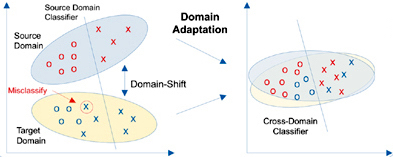
Fig 5. Domain adpation learns domain-invariant transformations and aligns domain distributions. Source image is from Fig. 1 in Choudhary2020, et al (2020), where domain adaptation is treated as a transductive transfer learning method. Here, this image illustrates the idea that covariate shift disappears once the different domains are aligned.
Essentially, both transfer learning and fine-tuning adapt the parameters learned from the source domain and seek further minimum adjustments to make the source and target domains comparable in the projection space (i.e., latent space) of the features. Like other domain adaptation approaches we’ve seen previously, this mitigates the covariate shift and allows the model to generalize to the target domain (Fig. 5).
$$ \text{Related tasks or domains} \xrightarrow{} P_\text{S} (X) \neq P_\text{T} (X) \xrightarrow[\text{fine-tuning}]{\text{transfer learning}} P_\text{S} (X’) = P_\text{T} (X’) $$
3. Domain Generalization when Target Domain is Inaccessible
So far, we have examined relatively simple OOD cases. However, more challenging scenarios can arise. In some instances, there might be no reliable prior information or even access to the target domain when training and locking the model for deployment. This challenge is often encountered in areas with limited training data and stringent regulations, where capturing a representative set becomes particularly difficult.
Machine learning literature uses the term domain generalization to characterize the goal of building robust models for target domains that are entirely inaccessible during model development. This presents a more challenging but potentially more needed extension of domain adaptation.
Apart from covariate shift, another OOD challenge we haven’t addressed is concept drift. It can seem daunting when the relationships between features and labels differ in the target and source domains, and this shift is unknown until after building, selecting, and deploying the models. Well, performance degrade in shifted target domain may not be a big issue in low-stakes scenarios, just further train the model or retrain. However, it’s a common challenge in healthcare, where AI/ML-based or AI/ML-derived products must meet primary and secondary goals in clinical trials for disease diagnosis and treatment.
So, what can we do in these more difficult cases? Consider a scenario where high school students are only allowed to take the real SAT test once. They should be allowed to take as many mocks as they want, right? Would that be helpful? I guess the more closely the mocks can reflect the real test, the higher the chance to achieve similar performance in the actual exam 3. Similarly, in domain generalization, we still need to think about how we can make the source domain data more like the target domain.
In the realm of concept drift, the relationships between Y and X are subject to change. In reality, there can also be situations where both P(Y|X) and P(X) change across domains. The key question is whether there are features or projections of features that establish a stable relationship with target labels, regardless of the domains.
3.1 Correlation vs Causality
In our quest for a more stable relationship between features and targets, let’s revisit how AI/ML models are trained.
Models utilize differences between model outputs and targets to update parameters. This leads to that fact that the model leverages the correlation between the features and targets to learn. A feature more correlated with the targets makes the model more likely to use it for predictions.
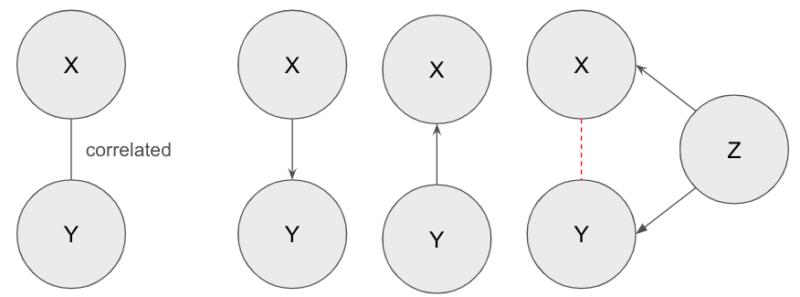
Fig 6. Correlation and causality. X and Y are two random variables that appear to be correlated. When digging into possible data generation process, it can be simplified as either they have a causal relationship or they have a common cause Z.
However, correlation is not a stable causal relationship; it can be spurious for various reasons such as sample collection biases. According to Reichenbach’s common cause principle (Hitchcock2021), if we observe a correlation or association between two random variables, it means either one of the variables causes the other or there is a third variable that causes both (known as confounding) (Fig. 6). Causal relationships are more stable than correlation, as spurious correlations can easily change across domains or environments.
For instance, consider a predictive model trained on medical data in the source domain, where an attribute like “number of hospital visits” shows a high correlation with disease outcomes due to selection biases. This attribute might seem crucial in the source domain, but once the selection biases disappear in the target domain, the correlation weakens, and the attribute loses its predictive power for disease outcomes. This scenario resembles a concept drift, highlighting opportunities to address OOD by identifying domain-invariant components in features that have a (ideally) causal relationship with target labels.
3.2 Multitask Learning and Adversarial Training
To identify invariant components in features, classical approaches like feature selection and engineering might come to mind. These handcrafted pre-processing methods rely on additional prior knowledge and are often employed in statistical learning and settings with small training sizes. However, such prior knowledge, acting as an inductive bias, may limit further performance improvements. For more complex problems with reasonable training sizes, we need an end-to-end training framework to learn invariant components in features with a stable relationship to target labels.
Multitask learning provides such a framework, allowing flexible representation learning. As depicted in the left part of Fig. 7, features can be encoded into a latent representation that predicts multiple attributes related to the main task (original target label) and auxiliary tasks (other attributes of sample instances). This facilitates the model to extract a more meaningful dense representation for predictions. Similar to Test-Time Training, well-designed auxiliary tasks can offer useful regularization on the networks, preventing overfitting on the main task.
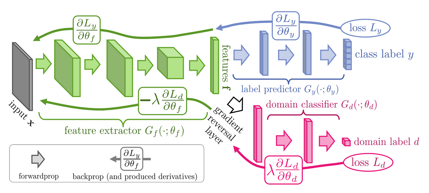
Fig 7. Domain-adversarial training a neural network that learns both class and domain label. A neural network can be divided into encoding and decoding parts. The left side illustrates a feature extractor $G_f$ encoding inputs $X$ into latent features $f$. The right side shows latent features $f$ being decoded to predict class label $y$ and domain label $d$. While the loss $L_y$ for the class label is normally backpropagated to update the whole network, the loss $L_d$ for the domain label needs to be reversed when used for adversarial training the feature extractor. Source image is from Fig1 in Ganin, et al (2016).
In situations with biased attributes showing high correlation with the target label (confounding), it’s crucial for the network not to exploit such shortcuts. Adversarial training becomes relevant in this context, as it can explicitly penalize any direct or indirect use of biased attributes and confounders. The right-hand side of Fig. 7 illustrates the decoding part in multitask learning along with adversarial training. The latent feature is used to predict both class label and domain label. However, since the domain label may introduce confounding effects, one may want the constructed latent space to be less predictive of the domain label. Thus, the prediction loss for the domain label is reversed during backpropagation to the encoding layers. This process is known as adversarial training and can be effective in mitigating known biases in the source domain if being well tuned. See eq3 for exact gradient descent operation for the whole training process in math4.
\begin{equation} \begin{align*} \theta_{y} &= \theta_{y} - \eta \frac{\partial L_y}{\partial \theta_{y}} \\\ \theta_{d} &= \theta_{d} - \lambda \frac{\partial L_d}{\partial \theta_{d}} \\\ \theta_{f} &= \theta_{f} - \left( \eta \frac{\partial L_y}{\partial \theta_{y}} - \lambda \frac{\partial L_d}{\partial \theta_{d}} \right) \end{align*} \end{equation}
Through these approaches, the goal is to find a more meaningful and less biased representation across domains, mitigating the concept drift issue.
$$ \text{Confounders, biases, etc} \xrightarrow{} P_\text{S} (Y|X) \neq P_\text{T} (Y|X) \xrightarrow{} P_\text{S} (Y|X’) = P_\text{T} (Y|X’) $$
Unlike domain adaptation seen previously, these approaches leverage previously ignored meta information that may reflect variance within the source domain itself. These methods don’t require access to the target domain at all, making them suitable for domain generalization. Moreover, they can be advantageous, especially when there’s no need for access to bias or sensitive attributes during inference in the target domain. On the flip side, these methods may involve more complex training and learning dynamics due to additional regularization terms.
3.3 Causality-inspired Representation Disentanglement and Invariant Risk Minimization
When performing representation learning, we can further ask if we can segregating a portion that holds more causal relevance to the target labels, and another portion that is closely associated with confounders or bias attributes. As discussed in the previous post of this series, a vision model trained on a source domain with images of cows on grassland may exhibit misclassification when confronted with a cow on ice (Causality2024). It’s obvious that the pixels of a cow should be a causal component for correct recognition of a cow while the pixels of background is related to the dataset biases (Fig. 8a).
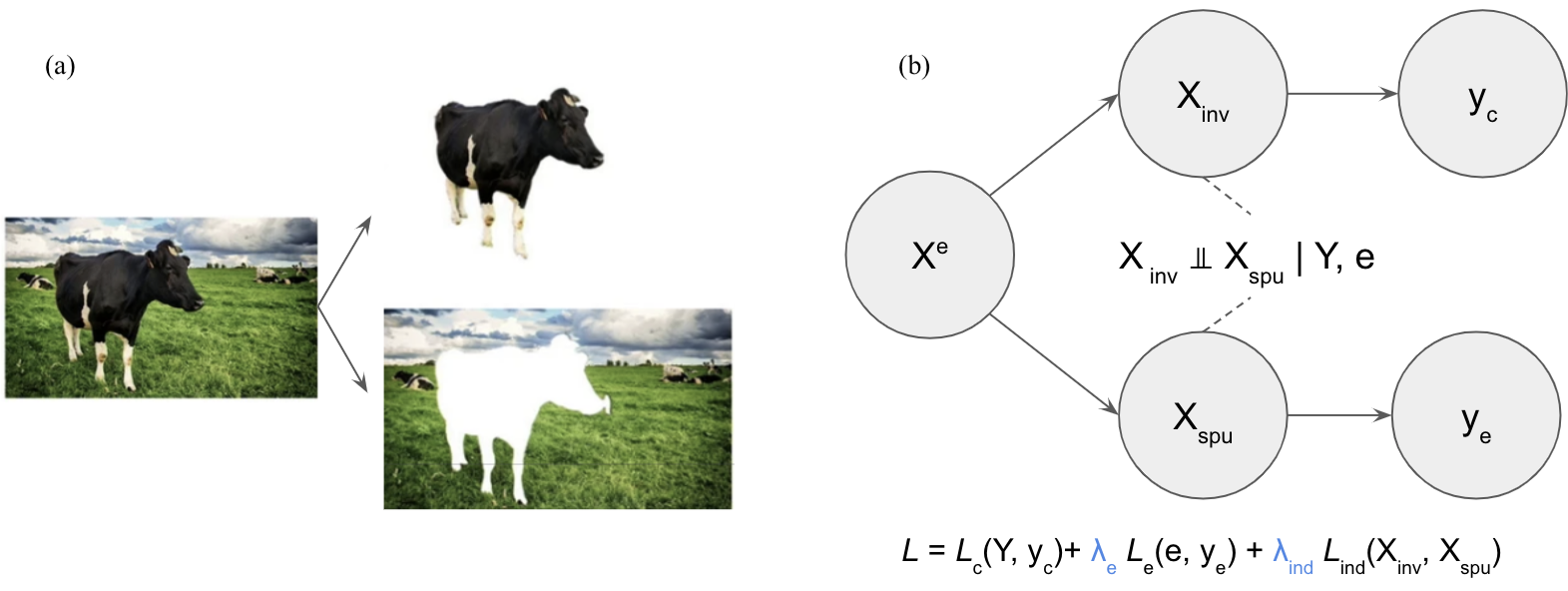
Fig 8. Illustration for Representation Disentanglement. (a) An image of a cow standing on a grassland can be decomposed into a cow and the background of the class land. For image recognition of a cow, the pixels of the cow are the causal factor with an invariant relationship with the concept label of a cow, while the background is with spurious correlation with the label of a cow. (b) Illustration for how causality-inspired representation disentanglement may look like. Raw inputs $X^e$ are encoded into $X_{\text{inv}}$ and $X_{\text{spu}}$, which are invariant across domains/environments (denoted as $e$) and spuriously correlated to environments, respectively. $X_{\text{inv}}$ and $X_{\text{spu}}$ should be independent from each other conditionally on the original class label $Y$ and environment $e$. Later, $X_{\text{inv}}$ and $X_{\text{spu}}$ are decoded to $y_c$ and $y_e$ for predicting the original class of interest and domain/environment label, respectively. This results in three loss terms, covering prediction errors for $Y$ and $e$ and conditional independence requirements. Source image is from a talk given by Koyejo in 2023ICML.
To address this, we can design the neural network to encourage disentanglement of the latent representation based on a causality-inspired decomposition (Fig. 8b). This approach is similar to the multitask learning framework discussed in last section, with the distinction that the latent space is now divided into two components. A key enhancement involves introducing a regularization term to promote the conditionally independent disentanglement of these components. This additional regularization ensures the separation of domain-invariant and domain-specific components during training. With the domain-invariant (hopefully causal) component from the latent representation space, we can now find a more stable $P(Y|X)$ across domains, mitigating the concept drift challenge.
$$ \text{Confounders, biases, etc} \xrightarrow{} P_\text{S} (Y|X) \neq P_\text{T} (Y|X) \xrightarrow{} P_\text{S} (Y|X_{\text{inv}}) = P_\text{T} (Y|X_{\text{inv}}) $$
Moving beyond disentanglement, the pursuit of fostering the invariance of learned representations across diverse domains or environments is encapsulated in Invariant Risk Minimization (IRM) (Arjovsky, et al (2019)). In contrast to the conventional training approach solely focused on minimizing empirical risk, known as Empirical Risk Minimization (ERM), as illustrated in more details in previous post, IRM takes a step further. By minimizing the risk across different environments, IRM renders the model less sensitive to variations that are irrelevant to the causal factors. The result is a representation that not only disentangles causal and spurious components but also ensures the invariance of causal components across diverse domains, thereby fortifying the model’s generalization capabilities. While IRM may only present significant improvement over EMR in scenarios involving anti-causal data-generation process (Wang & Veitch (2023)), IMR itself is so intriguing and worth a separate blog post or series in the future.
3.4 Multimodal Integration and Alignment
We’ve covered various tactics to enhance OOD robustness in AI/ML models. Let’s delve into one more tactic: Multimodal Integration and Alignment. This approach might not be commonly mentioned when talking about OOD robustness, but it’s an emerging strategy that proves effective. Before exploring the details of how Multimodal Integration and Alignment contribute to robustness improvement, let’s examine an example as shown below.
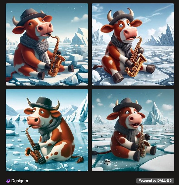
Fig 9. A cow playing saxophone on ice. Images were generated DALL·E 3.
Fig. 9 was generated by DALL·E 3 after receiving a text prompt of “a cow playing saxophone on ice” (link). Remarkably, the model behind DALL·E 3 seems to accurately understand various concepts, such as the cow, saxophone, and ice. This is particularly impressive given the fact that various biases present in real-world data and what such a prompt describes doesn’t exist in reality. The ML model involved in this example integrates two modalities: vision and text (Betker, et al (2023)). These modalities are integrated and aligned to match each concept before generating images based on the prompt. While the image generation part is beyond the scope of this post, multimodal integration and alignment represent a crucial tactic for enhancing the robustness of AI/ML models.
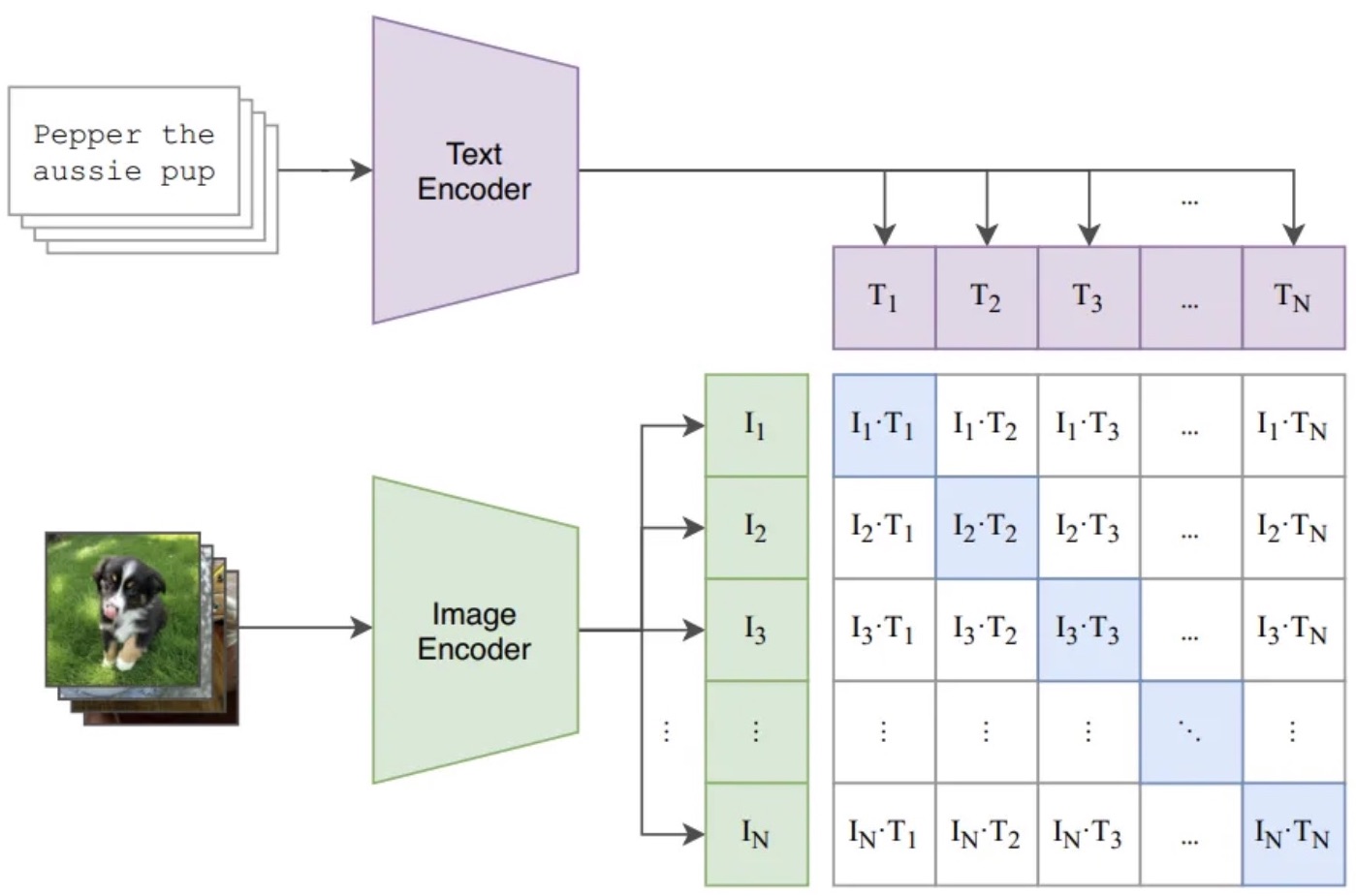
Fig 10. Contrastive Language-Image Pre-training. Source image from Fig 1 in Radford, et al (2021).
Fig. 10 illustrates Contrastive Language-Image Pre-training (CLIP), the core technique enabling vision-language integration and alignment in DALL·E. To achieve multi-modal pre-training, various images and their corresponding captions pass through an image encoder and text encoder, respectively. These encoders extract and represent the summary of information from an image $i$ and a caption $j$ as latent vectors $I_i$ and $T_j$, respectively. Training involves making the latent vectors for paired image and caption inputs ($I_i$ and $T_i$) as similar as possible, while for non-paired inputs, the vectors should be as different as possible. This process aligns the vision latent space with the text latent space, employing a contrastive learning strategy discussed in “How AI/ML Models Learn” in the last post (Xiao (2023)). CLIP leverages rich information from each modality input, capturing invariant concepts embedded in the latent space of the two modalities. Consequently, CLIP mitigates the concept drift issue. With such a pre-trained latent space, one can further conduct few-shot learning or zero-shot prediction.
3.5 Debiasing Training Tricks
In the previously discussed tactics, gradient-based learning plays a significant role. Several training techniques exist to mitigate biases in models during training. For instance, if positive and negative samples are known to be sampled from biased attribute groups, a practical approach is to design a batch sampler ensuring that all positive and negative samples within a batch originate from the same bias group. By doing so, backpropagated gradients merely reflect the target attribute of interest rather than those bias attributes.
However, when the bias attribute is unknown, alternative methods come into play. One strategy involves identifying bias groups based on the latent representations of samples during the learning process. By controlling learning dynamics or applying appropriate regularization according to the latent representations, the model can be adjusted to mitigate the adverse effects of spurious correlations between biased and target attributes. Given the length of this post, I recommend interested readers explore specific examples provided in references such as Yang2023, Hong2021 and Nam2020 for further insights into these debiasing techniques.
4. Concluding Remarks: The Pas de Deux of Data and Models
In this post, we explored various strategies to address out-of-distribution (OOD) challenges, encompassing both covariate shift and concept drift, in the pursuit of robust AI/ML models. Our discussion covered domain adaptation and domain generalization methods, considering scenarios with and without prior information about the target domain. At a high level, these strategies revolve around acquiring additional data or devising more suitable model training schemes.
Before concluding, it’s essential to reflect on the impact of data and model architecture on performance. The top panels in Fig. 11 illustrate different fitting conditions concerning model sizes. Panels A to C depict the classic bias and variance trade-offs, where the goal of statistical learning is to approach an ideal fit (i.e., ground truth) with a reasonable number of parameters. However, with the rise of deep neural networks and improved hardware capabilities, overparameterized models have become more prevalent (Panel D in Fig. 10). These models exhibit high learning capacity to directly fit every data point, showcasing the double-decent phenomenon (Nakkiran, et al. (2021)). This phenomenon challenges the conventional bias and variance tradeoff in statistical learning. However, what’s more important here is, this toy example suggests us two modeling options: ideal fit and direct fit when faced with data.
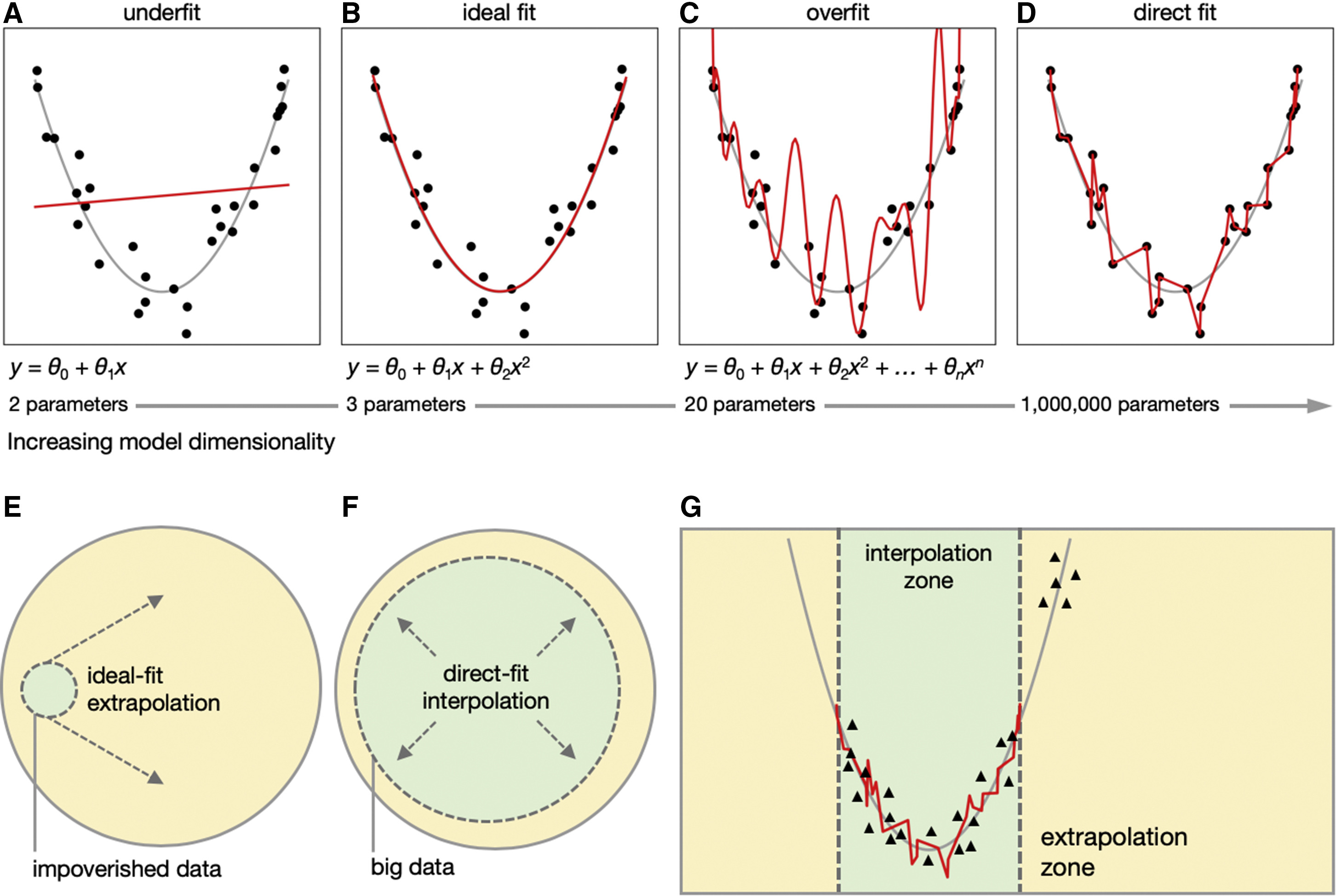
Fig 11. Double decent phenomenon and visualization of interpolation and extrapolation zoons. Source image from Fig. 1 in Hasson, et al (2020).
Meanwhile, when comparing the generalization in this toy case with the known ideal fit, we implicitly evaluate the accuracy of the model’s interpolation 5 and extrapolation 6. Extrapolation is generally more challenging and less accurate than interpolation, and OOD is more likely to occur in the extrapolation zone (Fig. 11G). Thus, achieving reliable extrapolation is crucial for OOD robustness. When dealing with impoverished data, seeking an ideal fit model with potential help from prior knowledge and inductive biases is still an attractive approach, especially considering its potentially better extrapolation ability compared to a direct-fit model. However, for cases with abundant data, the learning capacity of an overparameterized model may be appreciated more. Such a direct-fit on big data results in a larger interpolation zone and a smaller extrapolation zone, contributing to model robustness by relying more on interpolation than extrapolation (Fig. 11F).
Overall, for simple problems, an ideal fit model trained through appropriate learning strategies can provide reliable extrapolation for OOD. In more complex real-world problems, finding such an ideal fit model may be challenging. However, with rich data fed to overparameterized models, the interpolation zone becomes larger, and the model’s inability to extrapolate becomes less of a liability. This example underscores the complementary nature of models and data for generalization and robustness. Appreciating the pas de deux of data and models is crucial when building trustworthy AI/ML systems. Additionally, there are other requirements for trustworthy AI/ML, such as calibration/quality of uncertainty, fairness, explainability and transparency, and privacy, which will be explored in future discussions on the road to making model predictions trustworthy decisions.
Citation
If you find this post helpful and are interested in referencing it in your write-up, you can cite it as
Xiao, Jiajie. (Jan 2024). Toward Robust AI Part (2): How To Achieve Robust AI. JX’s log. Available at: https://jiajiexiao.github.io/posts/2024-01-06_how_robust_ai/.
or add the following to your BibTeX file.
@article{xiao2023howtoachieverobustai,
  title   = "Toward Robust AI Part (2): How To Achieve Robust AI",
  author  = "Xiao, Jiajie",
  journal = "JX's log",
  year    = "2024",
  month   = "Jan",
  url     = "https://jiajiexiao.github.io/posts/2024-01-06_how_robust_ai/"
}
References
-
Michielli, N., Caputo, A., Scotto, M., Mogetta, A., Pennisi, O. A. M., Molinari, F., … & Salvi, M. (2022). Stain normalization in digital pathology: Clinical multi-center evaluation of image quality. Journal of Pathology Informatics, 13, 100145.
-
Jong, J. (2017). Transfer learning: domain adaptation by instance-reweighting. Retrieved Jan 06, 2024, from https://johanndejong.wordpress.com/2017/10/15/transfer-learning-domain-adaptation-by-instance-reweighting/.
-
Lin, T. Y., Goyal, P., Girshick, R., He, K., & Dollár, P. (2017). Focal loss for dense object detection. In Proceedings of the IEEE international conference on computer vision (pp. 2980-2988).
-
Sun, Y., Wang, X., Liu, Z., Miller, J., Efros, A., & Hardt, M. (2020, November). Test-time training with self-supervision for generalization under distribution shifts. In International conference on machine learning (pp. 9229-9248). PMLR.
-
Choudhary, A., Tong, L., Zhu, Y., Mendelson, D., Rubin, D., Litjens, G., … & Zhu, J. (2020). Advancing medical imaging informatics by deep learning-based domain adaptation. Yearbook of medical informatics, 29(01), 129-138.
-
Hitchcock, C., & Rédei, M. (2021). Reichenbach’s Common Cause Principle (E. N. Zalta, Ed.). Stanford Encyclopedia of Philosophy; Metaphysics Research Lab, Stanford University. https://plato.stanford.edu/entries/physics-Rpcc/
-
Ganin, Y., Ustinova, E., Ajakan, H., Germain, P., Larochelle, H., Laviolette, F., … & Lempitsky, V. (2016). Domain-adversarial training of neural networks. Journal of machine learning research, 17(59), 1-35.
-
Causality for Machine Learning. Chapter 3: Causality and Invariance, Retrieved December 17, 2024, from https://ff13.fastforwardlabs.com/#how-irm-works.
-
Koyejo, S. (2023). On learning domain general predictors. https://icml.cc/virtual/2023/28441.
-
Arjovsky, M., Bottou, L., Gulrajani, I., & Lopez-Paz, D. (2019). Invariant risk minimization. arXiv preprint arXiv:1907.02893.
-
Wang, Z. & Veitch, V.. (2023). The Causal Structure of Domain Invariant Supervised Representation Learning. arXiv preprint arXiv:2208.06987.
-
Betker, J., Goh, G., Jing, L., TimBrooks, †., Wang, J., Li, L., LongOuyang, †., JuntangZhuang, †., JoyceLee, †., YufeiGuo, †., WesamManassra, †., PrafullaDhariwal, †., CaseyChu, †., YunxinJiao, †., & Ramesh, A. (2023) Improving Image Generation with Better Captions.
-
Chen, W., Wang, W., Liu, L., & Lew, M. S. (2021). New ideas and trends in deep multimodal content understanding: A review. Neurocomputing, 426, 195-215.
-
Radford, A., Kim, J. W., Hallacy, C., Ramesh, A., Goh, G., Agarwal, S., … & Sutskever, I. (2021, July). Learning transferable visual models from natural language supervision. In International conference on machine learning (pp. 8748-8763). PMLR.
-
Xiao, Jiajie. (Dec 2023). Toward Robust AI Part (1): Why Robustness Matters. JX’s log. Available at: https://jiajiexiao.github.io/posts/2023-12-17_why_robust_ai/.
-
Hasson, U., Nastase, S. A., & Goldstein, A. (2020). Direct fit to nature: an evolutionary perspective on biological and artificial neural networks. Neuron, 105(3), 416-434.
-
Nakkiran, P., Kaplun, G., Bansal, Y., Yang, T., Barak, B., & Sutskever, I. (2021). Deep double descent: Where bigger models and more data hurt. Journal of Statistical Mechanics: Theory and Experiment, 2021(12), 124003.
-
Yang, Z., Huang, T., Ding, M., Dong, Y., Ying, R., Cen, Y., … & Tang, J. (2023). BatchSampler: Sampling Mini-Batches for Contrastive Learning in Vision, Language, and Graphs. arXiv preprint arXiv:2306.03355.
-
Hong, Y., & Yang, E. (2021). Unbiased classification through bias-contrastive and bias-balanced learning. Advances in Neural Information Processing Systems, 34, 26449-26461.
-
Nam, J., Cha, H., Ahn, S., Lee, J., & Shin, J. (2020). Learning from failure: De-biasing classifier from biased classifier. Advances in Neural Information Processing Systems, 33, 20673-20684.
-
Focal loss adds a modulating term to conventional cross-entropy loss, focusing learning on hard misclassified examples. It dynamically scales the cross-entropy loss during the training process to penalize hard misclassified samples more than others (Lin, et al (2017)). ↩︎
-
Fine-tuning may be considered as a type of transfer learning method by people sometimes. By this definition, transfer learning may involves updating the weights of the pre-trained model as well. Meanwhile, the optional additional layers added in fine-tuning is also called adapters. Updating the entire pre-trained model can be computationally expensive due to its size, so a popular approach called efficient fine-tuning focuses on updating only the adapters. This trend has blurred the distinction between transfer learning and fine-tuning, and the terms are sometimes used interchangeably. I personally prefer to distinguish them a bit so that it can be clearer to readers how the training was actually done. ↩︎
-
One may also think about toughening the mock exams more than the actual test. This approach ensures that achieving high performance in the mock exams translates to good or even better performance in the real test. But here, consistent performance in mock exams and real test is emphasized. Thus similarity between mocks and real test are desired. ↩︎
-
$\eta$ and $\lambda$ in eq3 are two learning rates that update different modules in the network. ↩︎
-
Interpolation is the process of estimating values within the range of known data points. In the context of machine learning, it refers to predicting or estimating values for data points that fall within the observed range of the training data. ↩︎
-
Extrapolation, on the other hand, involves predicting values for data points that extend beyond the range of the observed data. It’s an extension of the model’s predictions beyond the range of the training data. ↩︎