Brilliant AI/ML Models Remain Brittle
Artificial intelligence (AI) and machine learning (ML) have garnered significant attention for their potential to emulate, and sometimes surpass, human capabilities across diverse domains such as vision, translation, and planning. The popularity of groundbreaking models like ChatGPT and Stable Diffusion has fueled optimism, with many speculating not if, but when, Artificial General Intelligence (AGI) will emerge.
Yet, beneath the in silico surface, AI/ML systems remain at their core parametrized mathematical models. They are trained to transform inputs into predictive outputs, which includes tasks like classification, regression, media generation, data clustering, and action planning. Despite the awe-inspiring results, the deployment of even the most sophisticated models reveals a fundamental fragility.
This fragility becomes apparent in terms of unexpected or unreliable predictions. For example, you may have experienced or heard that a chatbot spewing gibberish instead of useful information. This phenomenon is called hallucinations, where the model generates text that is irrelevant or nonsensical concerning the given inputs and desired outputs. Such hallucinations are arguably inevitable in auto-regressive large language models (LLMs).
The implications of this fragility are profound, particularly in risk-sensitive applications. Errors from the AI/ML systems can have severe consequences. In healthcare, a misdiagnosis by an AI-powered diagnostic tool or test can lead to severe impacts on patient health and quality of life. Similarly, in autonomous vehicles, a computer vision system’s failure to accurately detect objects can result in fatal accidents.
While AI/ML models often demonstrate impressive performance across numerous benchmarks during model development phases, these real-world errors persist. Degradation in performance, along with unforeseen errors, remains a significant challenge. As AI/ML technologies become increasingly integrated into society, the need for robust performance becomes paramount. The tremendous potential of AI/ML must be harnessed responsibly to ensure these models function reliably in the complex and dynamic real-world environment.
The Data Diet: How AI/ML Models Learn
To understand why AI/ML models can stumble, we need to slightly peek under the hood at how they learn. Think of it like training a personal chef: you provide them with recipes and feedback (labels or rewards), and they gradually figure out how to transform ingredients (inputs) into delicious dishes (outputs). With this analogy, we’ll see how major types of AI/ML models learn as below.
-
Supervised Learning: The most common approach, where you give the model both features (like image pixels) and labels (like “cat” or “dog”). The training process is to update the model parameters in order to reduce the error between the predicted outputs and the groundtruth labels. It’s like handing a chef a recipe book with labeled ingredients. While this method offers clarity and precision, acquiring annotated datasets can be costly.
-
Reinforcement Learning: A trial-and-error approach where the model explores and learns from rewards and punishments. Supervised learning also applies here, as the feedback from the reinforcement learning environment serves as labels, guiding the model to adjust its policy or value-action function for optimal long-term planning. Imagine a chef experimenting with different ingredient combinations without following a recipe and adjusting based on your reactions. That may be challenging since it requires you to taste all experimental dishes and share feedbacks.
-
Unsupervised Learning: Unlike supervised learning that finds the relationship between features and labels, unsupervised learning aims to extract inherent structures or patterns from unlabeled data. It’s like a chef intuitively discerning flavor profiles and accumulating, free from the constraints of explicit recipes or examination of ingredient labels. Unsupervised methods present their own set of challenges, as models must decipher complex data structures based on simply feature values.
-
Self-Supervised Learning: Cleverly design proxy tasks that help models learn without explicit labels, like masking parts of an image or sentence and asking the model to fill in the blanks. Alternatively, one can also train the model to assess if two augmented versions of an input originate from the same base in the latent projection space, which is also called contrastive learning. These are like challenging a chef to identify mystery ingredients or create dishes from a limited pantry, which trains the chef to understand relationships among ingredients, recipes and dishes. Afterwards, the chef can likely handle more abstract or more creative meal requests from you. The self-supervised learning method eliminates the need for labeled data by using the inherent structure of the data itself, enabling the model to learn a (compressed) representation that captures intrinsic patterns within the inputs. As a result, self-supervised learning becomes more and more popular than classic unsupervised learning these days.
Regardless of learning methods, in the training process, your AI chef is constantly adjusting their internal recipe book (model parameters) to improve their culinary skills. In other words, across these learning paradigms, a central tenet emerges: based on a set of training data, models continually adapt and refine their configurations, aiming to optimize alignment between their predictions and desired outcomes. But just like any human chef, they can be misled by faulty ingredients or biased information. Compared to the data used for model development, any discrepancies or shifts (i.e. so-called dataset shift (Hein2022)) in the distribution of data encountered during deployment may degrade performance. Unfortunately, as describing more in the next section, such dataset mismatch is common that results in AI/ML model fragility. We’ll delve deeper into these challenges, exploring the implications of distributional shifts and charting pathways to bolster AI model resilience.
Common yet Tricky Out-Of-Distribution
We’ve seen that AI/ML models are taught to align the model outputs to desired targets based on a specific set of training data (Fig. 1). This training paradigm helps the model find “optimal” parameter values, ensuring accurate alignment between predictions and targets. However, the effectiveness of AI/ML models hinges on the similarity between the test data and the training data. In essence, the more congruent the test data is with the training data, the more reliable the model’s performance tends to be. This effectiveness pattern is common in machine learning practice.
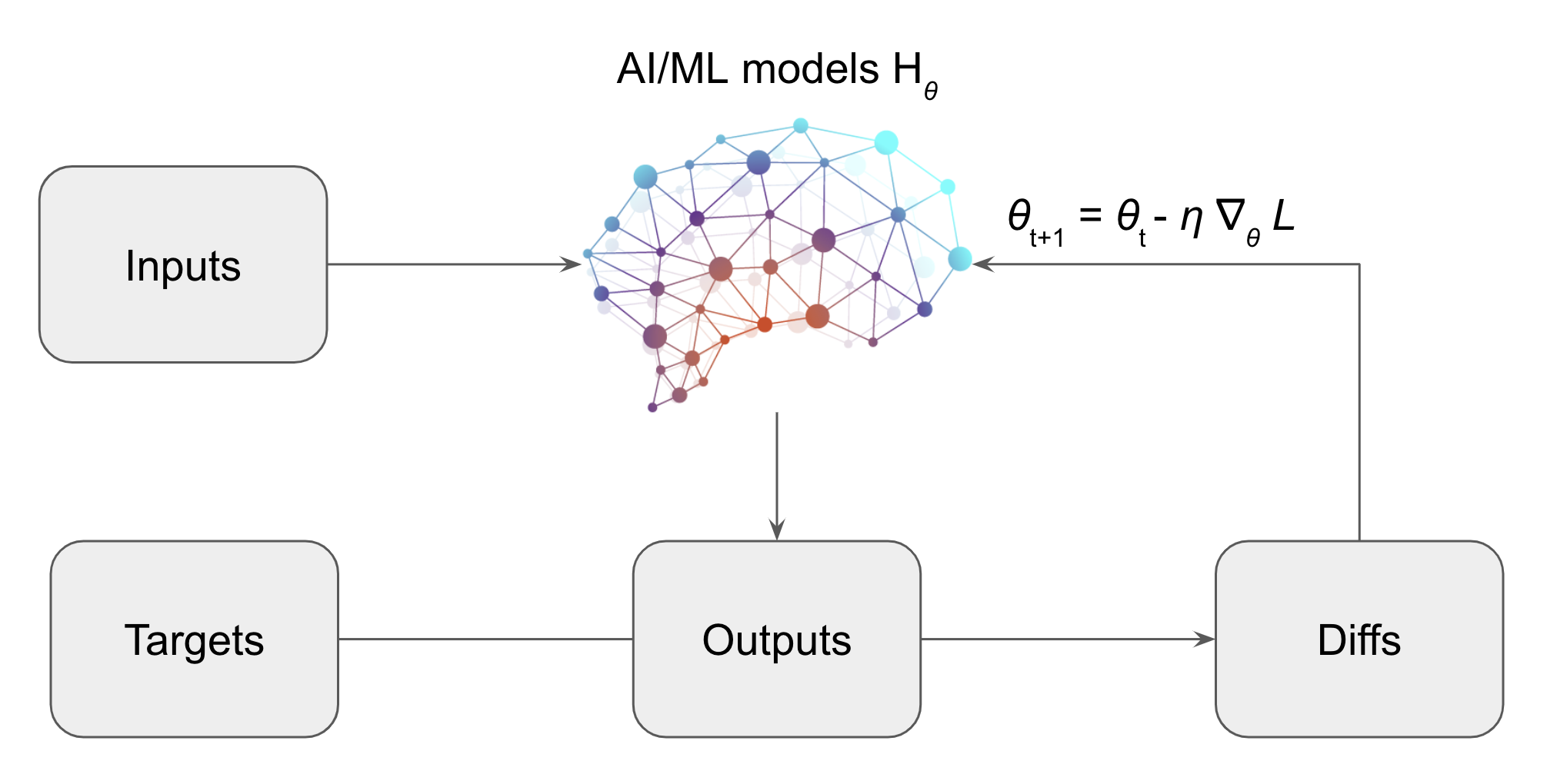
Fig 1. Illustration of AI/ML Model Learning Process. AI/ML models, represented as parameterized hypothesis functions Hθ, transform inputs X into outputs Hθ(X). Through iterative training and optimization, the parameters θ are adjusted to minimize the discrepancy L between the model’s outputs and the target values Y.
To explore this phenomenon further, let’s delve into the terminologies commonly employed in contemporary literature. The dataset used for training is referred to as the source domain, while the dataset used for testing is termed the target domain (Kouw2018). These datasets are typically categorized as either Independent and Identically Distributed (IID) or Out-of-Distribution (OOD) (Hein2022). It’s crucial to understand that the effectiveness pattern mentioned earlier, rooted in a fundamental principle of PAC learning 1, assumes optimal consistency between the test data and the training data (Mohri2018). This alignment of data distribution, often referred to as the IID assumption when deploying predictive models, is a benchmark for reliable model performance. However, real-world scenarios often deviate from this idealized setting, presenting challenges in model generalization for OOD data. For instance, an AI model trained exclusively on standard bacterial DNA might misclassify a novel bacterial species, mistaking it for a known variant, rather than acknowledging uncertainty (Ren2019). Likewise, image classifiers may falter when presented with objects in unfamiliar poses or contexts that deviate from their training data (like a cow on ice (Causality2024)).
Formally, IID and OOD are commonly defined by assessing the equality between the joint probability distributions of features and labels in both the source and target domains:
\begin{equation} \begin{aligned} \text{IID:} \quad P_\text{S} (X, Y) = P_\text{T} (X, Y) \end{aligned} \end{equation}
\begin{equation} \begin{aligned} \text{OOD:} \quad P_\text{S} (X, Y) \neq P_\text{T} (X, Y) \end{aligned} \end{equation}
This joint distribution can be deconstructed into the conditional probability, denoted as P(Y|X), which encapsulates the relationship between inputs X and targets Y, and the marginal probability P(X), which focuses solely on inputs. OOD scenarios predominantly manifest in two distinct forms 2:
- Covariate Shift: The conditional probability holds fixed across domains but input marginal probabilities differ. This is probably the most prevalent type of for OOD. For example, training data may lack samples for a particular feature range observed at test-time and thus make it hard for the model to reliably infer unseen regimes. (see toy example in Fig2). Covariate shifts are often seen when there are some selection biases or there are batch effects on the data generation processes.
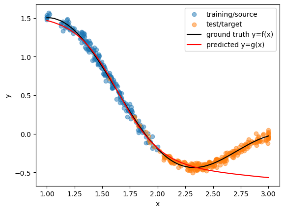
Fig 2. Model Behavior under Covariate Shift. In the source domain, data points with x > 2 are absent, whereas the target domain features numerous such instances. Consequently, the model’s performance is compromised for x > 2 in the target domain.
- Concept Drift: The conditional probability between inputs and targets itself shifts across domains, even if input distributions look similar. Relationships learned during training fail to transfer (see toy example in Fig3). Concept drift can be seen when there are any changes in mechanistic changes in the data generation process that may be even harder to anticipate in advanced compared to covariate shifts.
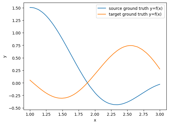
Fig 3. Model Behavior under Concept Drift. The relationship between x and y evolves across domains, rendering the previously learned model inadequate for the target domain.
While the landscape of OOD encompasses various nuanced scenarios (e.g. both P(Y|X) and P(X) may vary across domains), these two categories cover most common situations. As illustrated in Figs 2 and 3, even basic examples of covariate shift and concept drift can pose challenges. From a mathematical standpoint, it’s established that IID ensures consistent performance across both source and target domains. However, achieving such consistency in an OOD context proves more challenging. In moe details, a hypothesis model ℎ’s empirical risk 3 in the target domain, denoted as \( R_{\text{T}}(h) \) , can be estimated by the source domain loss ℓ weighted by the ratio between the joint distributions in the target and source domain as below:
\begin{equation} \begin{align*} R_{\text{T}}(h) &\equiv \sum_{y \in Y_{\text{T}}} \int_{\mathcal{X_{\text{T}}}} \ell(h(x), y) P_{\text{T}}(x, y) dx \\\ &= \sum_{y \in Y_{\text{T}}} \int_{\mathcal{X_{\text{T}}}} \frac{\ell(h(x), y) P_{\text{T}}(x, y)}{P_{\text{S}}(x, y)} P_{\text{S}}(x, y) dx \\\ &= \sum_{y \in Y_{\text{T}}} \int_{\mathcal{X_{\text{T}}}} \ell(h(x), y) P_{\text{S}}(x,y) \frac{P_\text{T}(x, y)}{P_\text{S}(x, y)} dx \\\ &\approx \frac{1}{n} \sum_{i=1, x_i \in \mathcal{X_{\text{S}}}, y_i \in Y_{\text{S}}}^{n} \ell(h(x_i), y_i) \frac{P_\text{T}(x_i, y_i)}{P_\text{S}(x_i, y_i)}. \end{align*} \end{equation}
As demonstrated by the equations above, achieving equality between the estimated target risk $\widehat{R}_{\text{T}}(h)$ and the estimated source risk \( \widehat{R}_{\text{S}}(h) \) typically requires \( P_{\text{T}}(x, y) = P_{\text{S}}(x, y) \) unless \( \ell_{\text{T}}(h(x), y) = \ell_{\text{S}}(h(x), y) = 0 \) .
In practice, while OOD scenarios are common, our goal remains: to achieve accurate and robust performance irrespective of whether we’re dealing with IID or OOD data. That is the requirement of robust AI/ML regardless of the IID or OOD. Consequently, the pursuit of designing AI/ML models that are resilient to a variety of OOD scenarios is crucial to ensure robust and dependable performance.
Summary
In wrapping up, this post has elucidated the foundational aspects of constructing compelling AI/ML models and shed light on the potential hurdles they encounter, particularly when confronted with OOD data. Understanding these challenges underscores the pressing need for robust AI. Ensuring that our AI systems can handle diverse and unexpected scenarios isn’t just a technical challenge—it’s crucial for their real-world applicability and trustworthiness. As we look ahead, bolstering AI’s resilience will be paramount. Join me in the forthcoming blog post, where we will explore in-depth strategies to fortify AI against these uncertainties and pave the way for more dependable and resilient machine learning solutions.
Citation
If you find this post helpful and are interested in referencing it in your write-up, you can cite it as
Xiao, Jiajie. (Dec 2023). Toward Robust AI Part (1): Why Robustness Matters. JX’s log. Available at: https://jiajiexiao.github.io/posts/2023-12-17_why_robust_ai/.
or add the following to your BibTeX file.
@article{xiao2023whyrobustness,
  title   = "Toward Robust AI (1): Why Robustness Matters",
  author  = "Xiao, Jiajie",
  journal = "JX's log",
  year    = "2023",
  month   = "Dec",
  url     = "https://jiajiexiao.github.io/posts/2023-12-17_why_robust_ai/"
}
References
-
Hein, M., Joaquin Quiñonero-candela, Sugiyama, M., Schwaighofer, A., & Lawrence, N. D. (Eds.). (2022). Dataset Shift in Machine Learning (Neural Information Processing). The MIT Press.
-
Mohri, M., Rostamizadeh, A. and Talwalkar, A. (2018) Foundations of Machine Learning. Cambridge, MA: The MIT Press. Chapter 2: The PAC Learning Framework, Available at: https://mitpress.ublish.com/ebook/foundations-of-machine-learning--2-preview/7093/9.
-
Kouw, W. M., & Loog, M. (2018). An introduction to domain adaptation and transfer learning. arXiv preprint arXiv:1812.11806.
-
Ren, J., Liu, P. J., Fertig, E., Snoek, J., Poplin, R., Depristo, M., … & Lakshminarayanan, B. (2019). Likelihood ratios for out-of-distribution detection. Advances in neural information processing systems, 32.
-
Causality for Machine Learning. Chapter 3: Causality and Invariance, Retrieved December 17, 2024, from https://ff13.fastforwardlabs.com/#how-irm-works.
-
PAC learning stands for Probable Approximately Correct (PAC) learning framework, which is a foundational concept in computational learning theory that provides guarantees on the generalization performance of a learner. ↩︎
-
The joint distribution of P(X, Y) can also be expressed in terms of P(X|Y) and P(Y). Thus, literature sometimes also mentions a third OOD scenario called label shift, meaning the P(Y) varies across domains while P(X|Y) stays stable. ↩︎
-
Empirical risk is a measure of the average loss incurred by a hypothesis model ℎ on a given dataset. In simpler terms, it quantifies how well a hypothesis fits the observed data. In a broader sense, the risk of a hypothesis ℎ is the expected loss it will incur when applied to new, unseen data, drawn from the underlying distribution. This is a measure of how well the hypothesis generalizes to new data. The empirical risk serves as an estimate or proxy for the true risk. When we train a model on a finite dataset, we compute its empirical risk to assess its performance on that dataset (Kouw2018). ↩︎